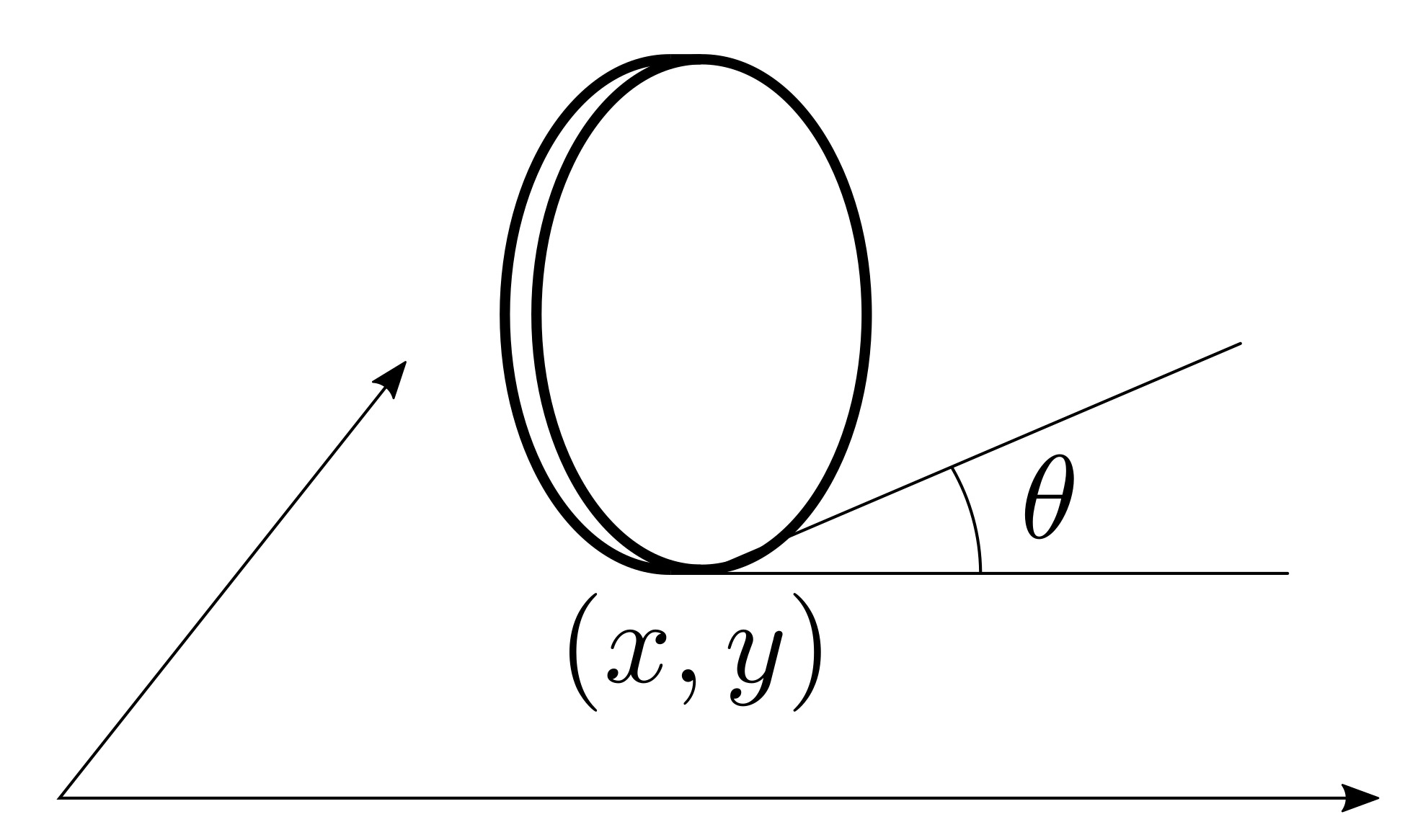
Unicycles are used to model a large variety of mobile robotic systems: ground, marine, and even aerial robots are very often abstracted using a rolling coin. The dynamic model of the unicycle is given by: $$ \begin{cases} \dot x = v \cos\theta\\ \dot y = v \sin\theta\\ \dot \theta = \omega, \end{cases} $$ where \(x\) and \(y\) are the coordinates of the position of the system in the plane, \(\theta\) is its orientation, and \(v\) and \(\omega\) are the linear and angular velocity control inputs. An effective way of designing controllers for unicycle models consists in controlling a point \(p\) at a distance \(l\) in front of the unicycle depicted in the following figure:
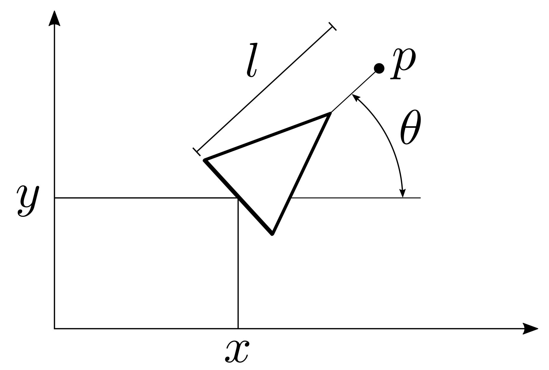
In fact, it is easy to see that $$ \dot p = \underbrace{\begin{bmatrix} \cos\theta & -\sin\theta\\ \sin\theta & \cos\theta \end{bmatrix}}_{R(\theta)} \underbrace{\begin{bmatrix} 1 & 0\\ 0 & l \end{bmatrix}}_{L(l)} \begin{bmatrix} v\\ \omega \end{bmatrix}. \tag{1} $$ So, once a controller for \(\dot p\) is designed, the inputs \(v\) and \(\omega\) to the unicycle can be easily computed as $$ \begin{bmatrix} v\\ \omega \end{bmatrix} = L^{-1}(l) R^T(\theta) \dot p. \tag{2} $$
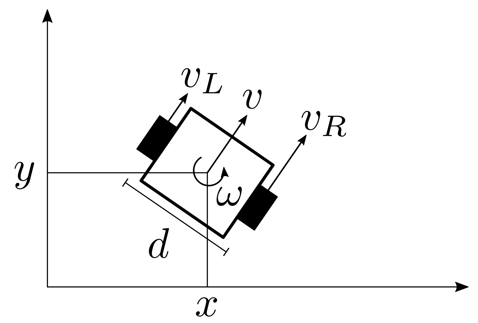
As in practice robots are not rolling coins, but rather have wheels, the values \(v\) and \(\omega\) can be turned into wheel speed in the case of differential-drive robots (shown in the figure above) as follows: $$ \begin{bmatrix} v\\ \omega \end{bmatrix} = \underbrace{\begin{bmatrix} \frac{1}{2} & \frac{1}{2}\\ -\frac{1}{d} & \frac{1}{d} \end{bmatrix}}_{D} \begin{bmatrix} v_L\\ v_R \end{bmatrix} \Leftrightarrow \begin{bmatrix} v_L\\ v_R \end{bmatrix} = D^{-1} \begin{bmatrix} v\\ \omega \end{bmatrix} \tag{3} $$ Among the ground mobile robots modeled as unicycles there is the differential-drive brushbot, which implements a peculiar locomotion strategy that leverages brush elements to turn vibration into locomotion. The locomotion principle is very simple and thus renders the brushbot robust to interactions with the environment, including external objects or other brushbots. The motion is achieved by bouncing at a very fast pace on very small pogo sticks (the brushes). And just like with pogo sticks, if you lean forward, you can only move forward. Thus we need a more sophisticated method to properly control these Hemingwayian unicycles.
To start off, one could consider a version of the unicycle constrained by \(v\ge0\), only non-negative linear velocities allowed, and employ the following controller: $$ \begin{bmatrix} v^\star\\ \omega^\star \end{bmatrix} = \arg\!\min_{v,\omega} \left\{ \left\| \begin{bmatrix} v\\ \omega \end{bmatrix} - L^{-1}(l) R^T(\theta) \dot p \right\|^2 ~\colon~ v\ge0\right\} \tag{4}, $$ which is a mouthful for:
The problem with this is that, because of its construction, the differential-drive brushbots cannot turn in place: \(\omega\neq0\implies v\neq 0\). This again is due to the fact that each brush cannot move backward, which is not equivalent to \(v\ge0\), but rather to \(v_L\ge0\) and \(v_R\ge0\) in (3).
Enforcing the constraints \(v_L\ge0\) and \(v_R\ge0\) might lead to the practical impossibility of moving under arbitrary \(\dot p\), since, intuitively, not all possible \(v\) and \(\omega\) are simultaneously realizable. To circumvent this issue, we need more degrees of freedom: the idea is that of allowing the distance \(l\) to change, and finding its optimal value subject to the constraints that \(v_L\ge0\) and \(v_R\ge0\). If \(l\) can change over time, (1) becomes $$ \dot p = R(\theta) L(l) D \begin{bmatrix} v_L\\ v_R \end{bmatrix} + \underbrace{\begin{bmatrix} \cos\theta\\ \sin\theta \end{bmatrix}}_{r(\theta)} w, $$ where (3) was substituted in, and \(w\) is the rate of change of \(l\), which is now an additional control input.
Although \(l\) is changing, we might want to drive it, through \(w\), to a desired value \(\bar l\). Moreover, we would like to keep it positive and less than \(\bar l\). The stated conditions lend themselves to be encoded using a control Lyapunov function (CLF) and a control Barrier function (CBF). CLFs and CBFs are control-theoretic tools which allow us to ensure stability and safety of dynamical systems. In this case the dynamical system is simply $$ \dot l = w, $$ and the stability and safety constraints are
respectively. To this end, we define the following CLF and CBF:
Without going too much into the technical details, it suffices to say that using \(V\) and \(h\) we can turn stability and safety conditions into constraints on the control input \(w\), the rate of change of \(l\). These constraints can be then included in an optimization-based formulation as follows: $$ \begin{aligned} \underset{v_L, v_R, w, \delta}{\mathrm{minimize~}} & \left\| \begin{bmatrix}R(\theta) L(l) D & r(\theta)\end{bmatrix} \begin{bmatrix}v_L\\v_R\\w\end{bmatrix} - \dot p\right\|^2 + \delta^2\\ \mathrm{subject~to~} & v_L\ge0\\ & v_R\ge0\\ & \frac{\partial V}{\partial l} w \le -V(l) + \delta\\ & \frac{\partial h}{\partial l} w \ge -h(l), \end{aligned} \tag{5} $$ which is a convex quadratic program and, as such, can be solved very efficiently in order to evaluate the values of the control inputs \(v_L\) and \(v_R\). \(\delta\) is just a slack variable which allows us to prioritize the safety constraint (enforced using \(h\)) over the stability constraint (enforced through \(V\)), by relaxing the latter. The results of the application of the described controllers are shown in the following simulation videos.
In all the cases, the differential-drive robot, represented by an arrow, is controlled to drive to the black dot using a simple proportional controller on \(p\), the tail of the arrow. Notice how in the first video, the robot moves backwards at the beginning of the trajectory as a result of the mapping (2). As this would be impossible to realize with Hemingwayian brushbots, in the second video, the linear velocity is thresholded at 0 according to (4). Nevertheless, in the first part of the trajectory, the robot still turns in place, which, as discussed above, leads to negative wheel velocities. Therefore, in the last video, the controller solution of (5) is used: at the beginning \(l\) is reduced (as shown by the length of the arrow and highlighted by the red dot) in order to ensure the \(v_L\) and \(v_R\) are always positive. The desired value of \(l\), \(\bar l\) (indicated by the green dot), is tracked as a result of the constraints in (5).
What is Hemingwayian about these unicycles?
"Write drunk, edit sober" is a quote attributed to Ernest Hemingway. Despite its faithfulness and authenticity, separating writing from editing has been shown to be an effective technique for good writing. As a result, many text editors (such as ghostwriter and atom) have introduced Hemingway modes, where backspace and delete keys are disabled and it is only possible to add text at the end of a document. This way, you are forced to avoid editing and to only write, to only make forward progress.
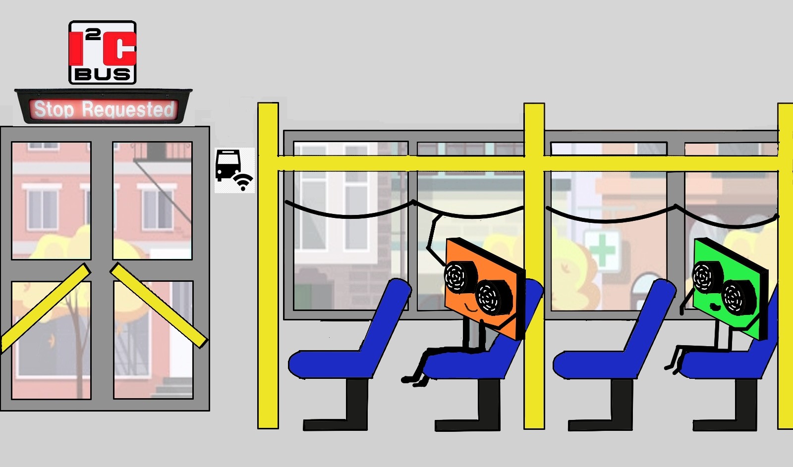
When I first hopped on a bus in the U.S., I was shocked by the rudimentality of the contraption typically used to request a stop, consisting in a string running from the front to the the back of the bus which is to be pulled down (see the cartoon above). Yet, this effective passenger-driver communication modality shares the same working principle with the I2C, a two-wire interface which allows microcontrollers, actuators and sensors to talk to each other in many robotics applications. One of these applications is the brushbot where distance sensors and other peripherals communicate with the main microcontroller using the I2C protocol.
In the early stages of development of the brushbot, we manufactured a prototype with 8 time-of-flight sensors arranged all around the robot in order to detect obstacles and other robots in the environment. Manual surface mount was challenging and, out of 8, we managed to get 2 sensors properly soldered. Nevertheless, after testing them, we were not able to communicate with either of them and get meaningful distance readings. We tried all sorts of software-based approaches, but, for the life of us, we could not read a single bit.
Then, one day, looking more closely at the circuit schematic, the epiphany: too much pull up!
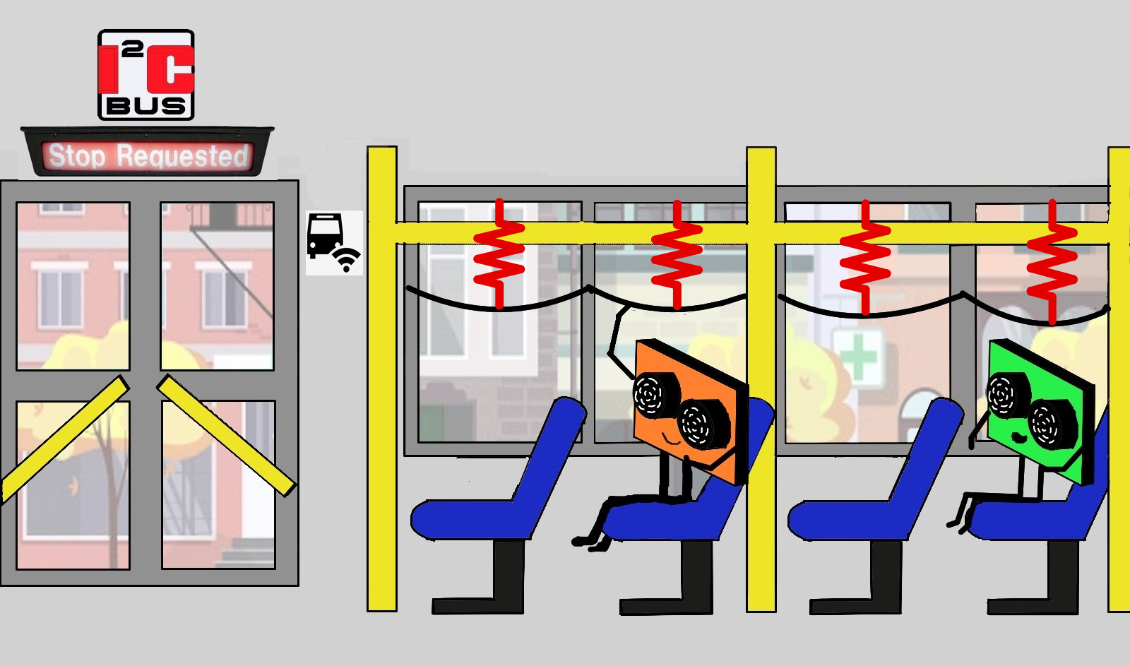
Drawing an analogy with the way of requesting a stop in the bus, the time-of-flight sensors were sitting between two wires, ground (GND) and serial data (SDA). The former is connected to a reference of low voltage, the latter—the string to request the bus stop—to a high voltage (VCC). In order to communicate with the microcontroller, each sensor has to pull down the SDA line to GND in a specific pattern, defined by the I2C protocol. The problem was that the SDA line was pulled-up to VCC with resistors of too small resistance. This is analogous to having the string to request a stop connected to the ceiling of the bus with very stiff springs. The poor sensors were unable to ground the SDA line, be heard by the driver, and thus got stuck in the bus.
My favorite interpretation of Eduardo Scarpetta's play "Miseria e nobiltà" ("Poverty and Nobility") is the one by Totò, the Prince of laughter. The video above shows an extract from the comedy film taken from the play in which Totò pronounces the words "la migliore non c'è" ("the best is not there"), speaking about chairs in his house. I find this line hilarious for its spectacular absurdity.
It is evident that, among the chairs of a house, there must be the best one, although this might not be unique. In fact, if we let \(S\) be the non-empty finite set of chairs in a house, we can show by induction that it contains its supremum, \(\sup S\), namely there is a best chair.
as \(x^\prime \in S^\prime \subseteq S\) and \(x \in S\).
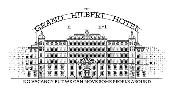
Would the line "la migliore non c'è" still sound spectacularly absurd if Totò lived in the Grand Hilbert Hotel assuming there is a chair in each room? And what if the 1st room contains 1 chair, the 2nd contains \(\frac{1}{2}\) chair, the 3nd contains \(\frac{1}{3}\) chair, and so on?
Conservation theorems play a fundamental role in physics. In particular, their connection to symmetry in classical and quantum mechanics is a beautiful manifestation of the interconnection between mathematics and physics.
Among the notoriously conserved quantities, there is the angular momentum (in absence of externally applied torques). For a rigid body with inertia matrix \(I\) and angular velocity \(\omega\), the angular momentum is given by $$ L = I \omega, $$ while the kinetic energy can be expressed as $$ T = \frac{1}{2} \omega^T I \omega. $$ The relation between angular momentum and kinetic energy is then: $$ \begin{aligned} \nabla T = L. \end{aligned} $$
What is fascinating about this relation is that \(\nabla T\) corresponds to the direction orthogonal to the plane tangent to the so-called inertia ellipsoid associated with the inertia matrix \(I\) at \(\omega\). And this direction turns out to be equal to \(L\). As \(L\) is a conserved quantity, this direction doesn't change. Moreover, it can be shown that the distance \(d\) between the center of the inertia ellipsoid (the center of mass of the rigid body) and the tangent plane is equal to $$ d = \frac{2T}{\|L\|}, $$ which is also constant, as \(T\) and \(L\) are both conserved in absence of externally applied torques. Therefore, the plane orthogonal to \(L\) and tangent to inertia ellipsoid is called the invariable plane.
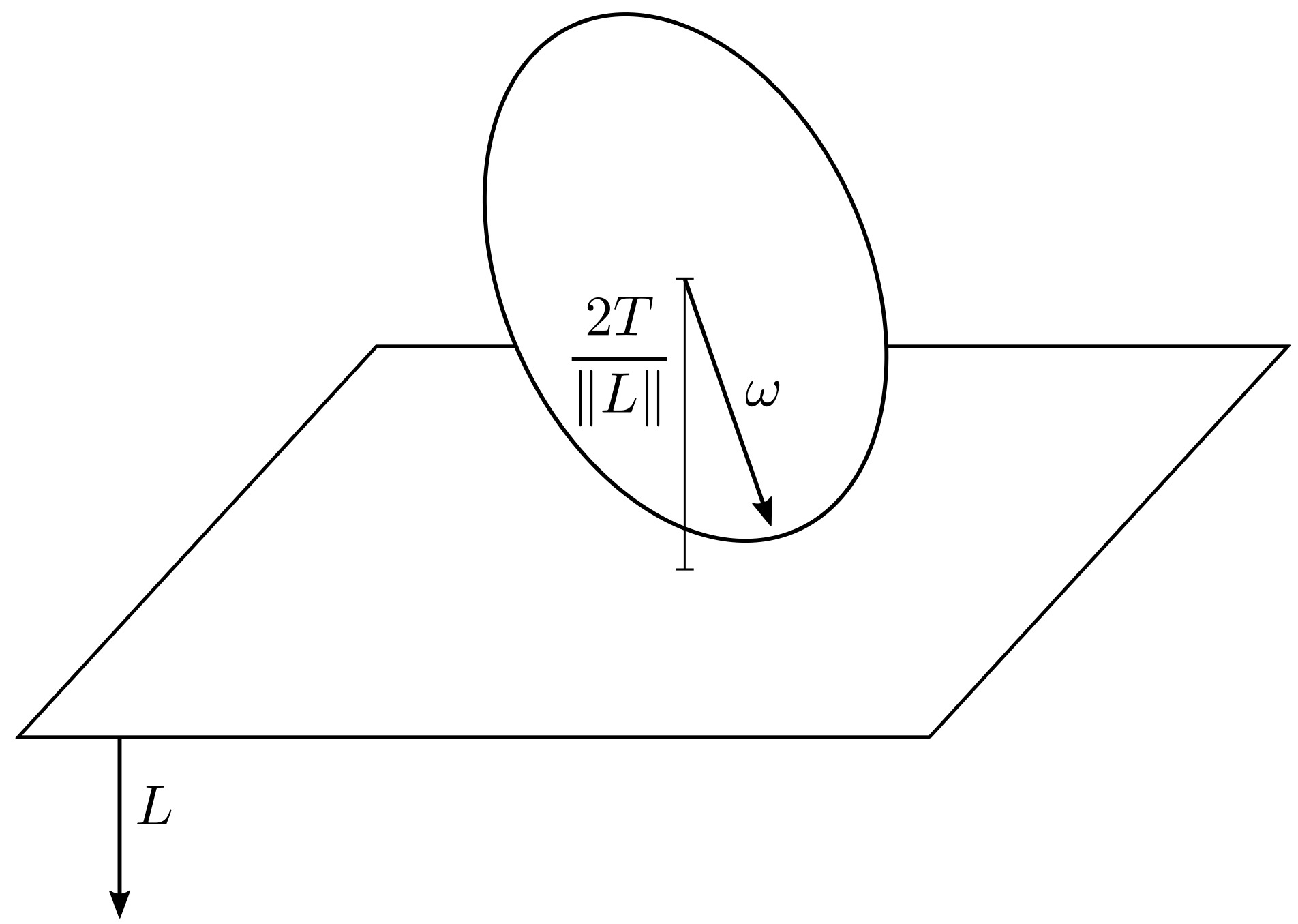
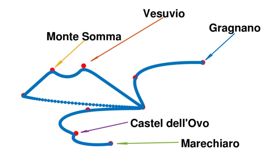
The Poinsot's construction summarizes these two properties in a very elegant way. Consider the motion of a rigid body with given inertia matrix and initial angular momentum. With no external torques applied, the angular momentum is conserved. Now consider the inertia ellipsoid as a real body (e.g. an easter egg) placed on the invariable plane. Then, the motion of the rigid body corresponds to the inertia ellipsoid rolling without slipping on the invariable plane. In fact, as the inertia ellipsoid is tangent to the invariable plane at \(\omega\), the contact point between the ellipsoid and the plane is instantaneously stationary, which is the condition for rolling without slipping.
Three disciplines an aspiring control engineer should learn about are Linear Control Systems, Nonlinear Control Systems and Optimal Control. I had the pleasure of taking a course on Optimal Control with the inspiring Magnus Egerstedt. The idea of using Angry Birds to study and demonstrate the use of optimal control came, in fact, from one of his lectures.
Two canonical problems in optimal control are:
Given a dynamical system, the initial conditions optimization problem consists in finding the best initial conditions, i.e. those that minimize a desired cost defined to achieve a desired objective. In switching time optimization, the goal is to minimize a cost functional by varying the switching times between a collection of given system dynamics.
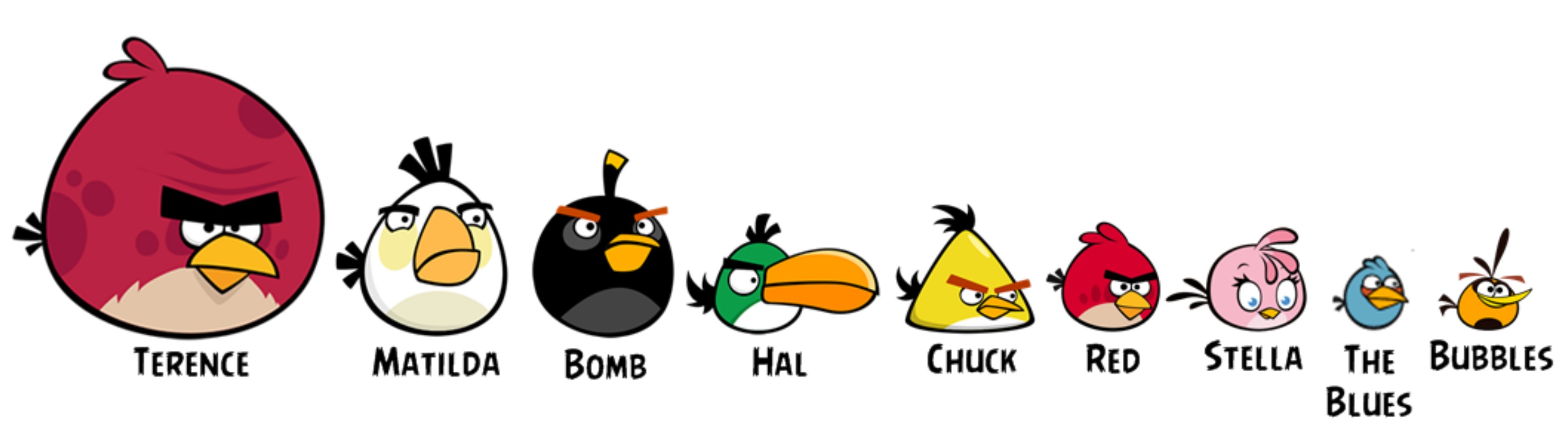
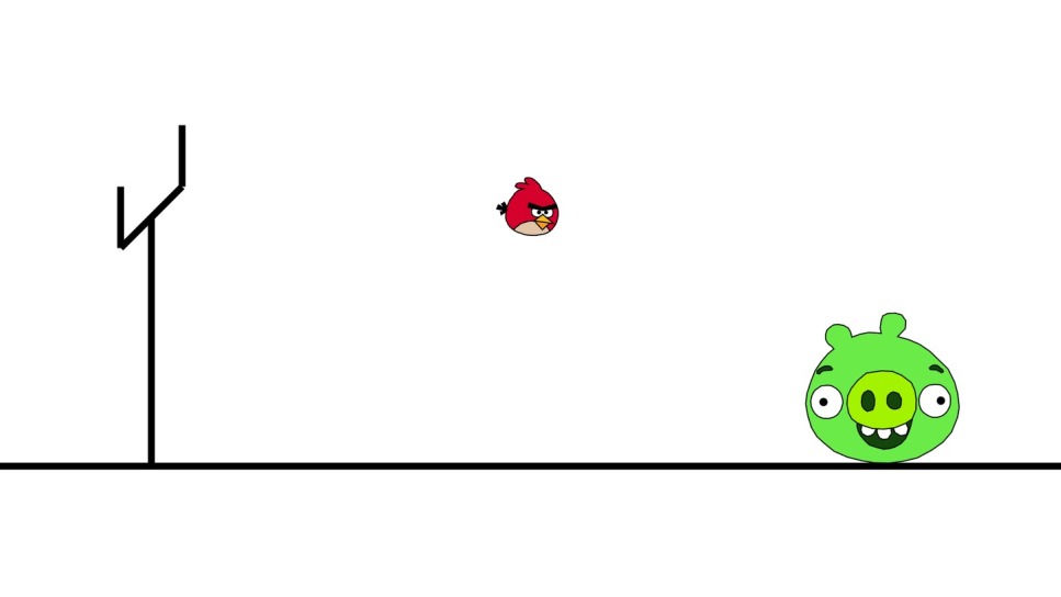
The subject perfectly lends itself to being explained by and applied to the famous video game Angry Birds. The game consists in throwing birds with a sling with the goal of killing pigs that are present in the environment.
In the case of the bird "RED" (see figure above), the goal is to pick the optimal initial conditions, namely speed and direction of the throw, to kill the pigs. The bird "CHUCK" has the ability of instantaneously increasing its speed, therefore the goal is that of picking the optimal time to switch to the accelerated mode.
The code to simulate these two problems and to play Angry Birds using MATLAB can be found here.
Oscar 'o SCARA is an audacious SCARA robot, and the protagonist of a journey in the wonderful world of robot control. Oscar's adventures range from robot manipulator kinematics and dynamics, to position and force control.
This was actually the final project of the course Robot Control taught by Prof. Bruno Siciliano at the Università degli Studi di Napoli Federico II. The PDF of the project report can be downloaded here. A teaser is shown in the video below.
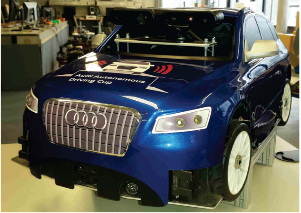
The Audi Autonomous Driving Cup is a student competition where the goal is to develop algorithms required to render a small-scale RC vehicle fully autonomous and able to navigate a city-like scenario following a given list of maneuvers. The hardware platform used is a 1:8 model vehicle developed by Audi specifically for the contest.
In 2015, Konstantin Andreev, Sinan Hasirlioglu, Eduardo Morales, Parthasarathy Nadarajan and I, under the supervision of Prof. Michael Botsch, participated, as the team leTHItdrive of the Technische Hochschule Ingolstadt, in the first edition of the Audi Autonomous Driving Cup.
We won the Open Challenge with the performance of a car that was able to autonomously kick a ball into a goal by drifting (see videos below), and scored 4th overall behind Technical University of Munich, Karlsruhe Institute of Technology and University of Freiburg!
The PDF of a short presentation describing the architecture of our vehicle's control system can be downloaded here.
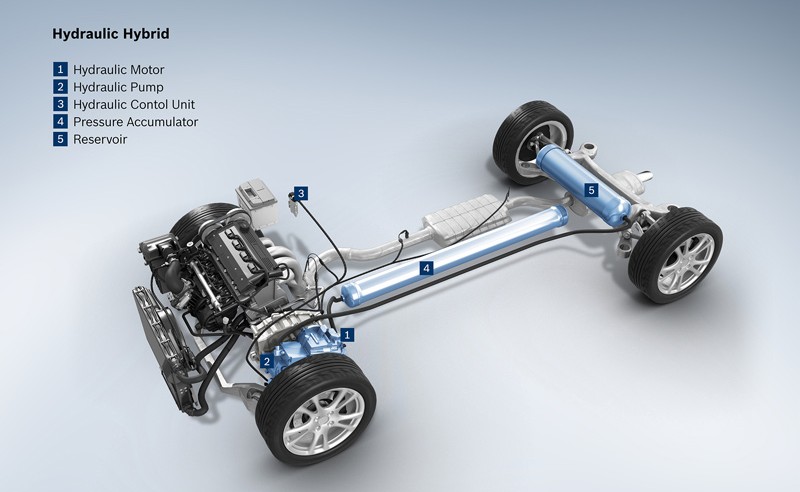
As an exercise in modeling complex and interconnected dynamical systems, this project aims at analyzing the performance of an hydraulic hybrid vehicle in terms of fuel consumption when compared to traditional internal-combustion-engine-based vehicles.
The analyses have been carried out using MATLAB/Simulink, and here you can find the code to simulate urban and extraurban driving cycles to assess fuel economy in passenger cars.